Phase Estimation Accuracy Tab
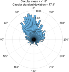
The “Phase Estimation Accuracy” tab measures the accuracy of the autoregressive forward prediction algorithm.
Oscillation Panel
Choose which oscillation to display phase estimation accuracy metrics for.
Offset Samples
Adjust the number of offset samples so that mean phase estimation error is aligned at 0 degrees.
Update
Calculate new phase estimation accuracy metrics for the current time period. The metrics do not continuously update. You must click "Update" for updated metrics. Metrics are run on the most recent ten seconds of data, stored in a buffer (the length of data stored in the buffer is configurable in the "Advanced" tab.)
Clear
Clear the buffer. This can be helpful if disturbance or major artifact occurred within the data stored in the buffer (default is ten seconds) and you do not want that disturbance included in the calculations.
Phase Error
To target a specific phase within a target frequency, you must predict the phase shortly into the future. This is because it takes some time to perform calculations and generate, send, and receive triggers. The bossdevice is continuously predicting the phase of the target frequency band. (This is what is displayed in the Phase plot under the "Oscillations" tab.)
The buffer maintains a ten-second period (configurable in the “Advanced” tab) of the data. The bossdevice continuously updates the buffer as new data comes in (i.e., the buffer will always have the most recent ten seconds of data). When “Update” is pressed, the bossdevice will compare the phase of the predicted signal with the phase of the real signal at a random point during each period. (i.e., for 10 seconds of data with alpha as the frequency of interest, there will be 100 periods and, therefore, 100 comparison points.)
Because the signal is a complex biosignal mixed with noise, the autoregressive forward prediction algorithm is imperfect. At each comparison point, the “Phase error”, a measure of how early or late the predicted phase is compared to the real phase, is calculated. The error is then plotted on a polar histogram in bins of five degrees. A perfect phase estimation would result in an error of 0 degrees, and in cases where phase estimation accuracy was high, the error would be centered around 0 degrees. In cases where phase estimation accuracy was low, the error would be distributed or random throughout the plot. The height of each bin shows which percentage of the observations in this 10-second window had the given error.

Circular Mean and Standard Deviation
The “Circular Mean” (displayed above the plot once “Update” has been clicked) is the mean phase error. If the circular mean is between 0 and 180 degrees, the predicted phase is, on average, early compared to the real phase. If the circular mean is between 180 and 360, the predicted phase is, on average, late compared to the real phase. A mean of 5 degrees would be less early than 150 degrees, and a mean of 335 degrees would be less late than 185 degrees. The “Circular Standard Deviation” (also displayed once clicked) is the standard deviation of the circular mean.
Notes
- Phase Estimation Accuracy does not measure how accurate the TMS pulse was to the target phase.
- The "Clear" button empties the buffer. "Update Spectrum" cannot be pressed until a minimum data threshold is present in the buffer.
- The Spectrum Buffer and the Phase Estimation Accuracy Buffer are independent; clearing one will not clear the other.
Common Causes of High Phase Error
If the phase error is high, it could be due to poor signal quality, improperly configured thresholds, spatial filter design, or individual differences in the strength of the target signal.
Poor Signal Quality
- Are your electrodes prepared well? Are impedances low? Are ground and reference working properly?
- Is there a large amount of electromagnetic noise in your recording space? Common sources include electronic devices, electrical outlets, incandescent lights, CRT monitors, and intercom systems, among many others.
- Is your subject uncomfortable? If so, they may move frequently or tense their muscles.
Improperly Configured Thresholds
Clean Signal Status relies on four thresholds that must be tuned to each session. The first two, “Eyeblink” and “Range,” are configurable in the “Artifacts” tab. The third and fourth, the min and max “Range,” are configurable in the “Oscillations” tab.
The default values for these thresholds are set to always be met. However, appropriate values for these thresholds will vary by person and protocol. Generally, setting the thresholds so that “Clean Signal Status” stays green for 5 seconds is appropriate.
Spatial Filter Design and Individual Differences
A spatial filter design attempts to isolate a signal of interest at a specific location on the scalp. Some signals are strong, and some are weak. A spatial filter design can strengthen or weaken these signals. Individual variability in the strength and location of a given signal confounds this. It is possible that not all subjects will have a given signal at a given location with a given spatial filter.